Compute and display a univariate averaged shifted histogram (polynomial kernel)

See bin1 & ash1 for more information.

stat_ash(mapping = NULL, data = NULL, geom = "area",
  position = "stack", ab = NULL, nbin = 50, m = 5, kopt = c(2,
  2), na.rm = FALSE, show.legend = NA, inherit.aes = TRUE, ...)

Arguments

mapping	Set of aesthetic mappings created by aes() or aes_(). If specified and inherit.aes = TRUE (the default), it is combined with the default mapping at the top level of the plot. You must supply mapping if there is no plot mapping.
data	The data to be displayed in this layer. There are three options: If NULL, the default, the data is inherited from the plot data as specified in the call to ggplot(). A data.frame, or other object, will override the plot data. All objects will be fortified to produce a data frame. See fortify() for which variables will be created. A function will be called with a single argument, the plot data. The return value must be a data.frame, and will be used as the layer data.
geom	Use to override the default Geom
position	Position adjustment, either as a string, or the result of a call to a position adjustment function.
ab	half-open interval for bins [a,b). If no value is specified, the range of x is stretched by 5% at each end and used the interval.
nbin	number of bins desired. Default 50.
m	integer smoothing parameter; Default 5.
kopt	vector of length 2 specifying the kernel, which is proportional to ( 1 - abs(i/m)^kopt(1) )i^kopt(2); (2,2)=biweight (default); (0,0)=uniform; (1,0)=triangle; (2,1)=Epanechnikov; (2,3)=triweight.
na.rm	If FALSE, the default, missing values are removed with a warning. If TRUE, missing values are silently removed.
show.legend	logical. Should this layer be included in the legends? NA, the default, includes if any aesthetics are mapped. FALSE never includes, and TRUE always includes. It can also be a named logical vector to finely select the aesthetics to display.
inherit.aes	If FALSE, overrides the default aesthetics, rather than combining with them. This is most useful for helper functions that define both data and aesthetics and shouldn't inherit behaviour from the default plot specification, e.g. borders().
...	Other arguments passed on to layer(). These are often aesthetics, used to set an aesthetic to a fixed value, like colour = "red" or size = 3. They may also be parameters to the paired geom/stat.

Details

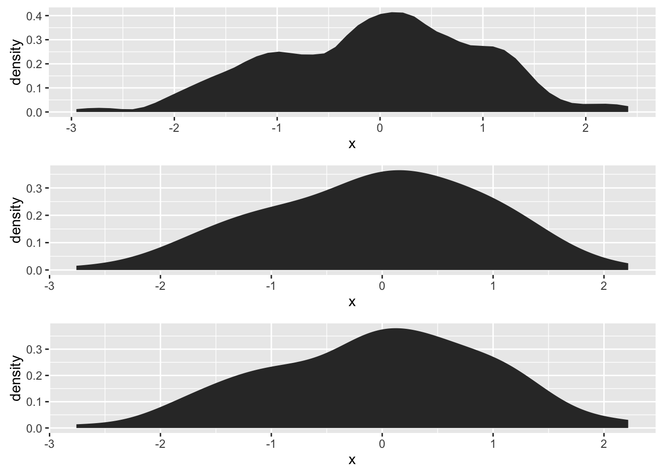
A sample of the output from stat_ash():

Aesthetics

geom_ash understands the following aesthetics (required aesthetics are in bold):

• x

• alpha

• color

• fill

• linetype

• size

Computed variables

density

ash density estimate

References

David Scott (1992), "Multivariate Density Estimation," John Wiley, (chapter 5 in particular).

B. W. Silverman (1986), "Density Estimation for Statistics and Data Analysis," Chapman & Hall.

Examples

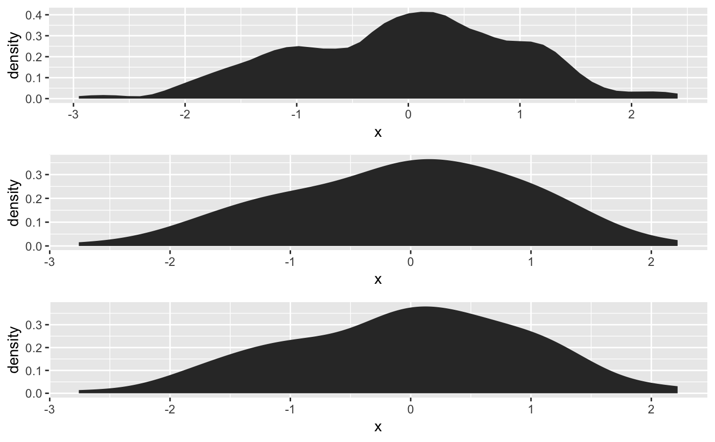
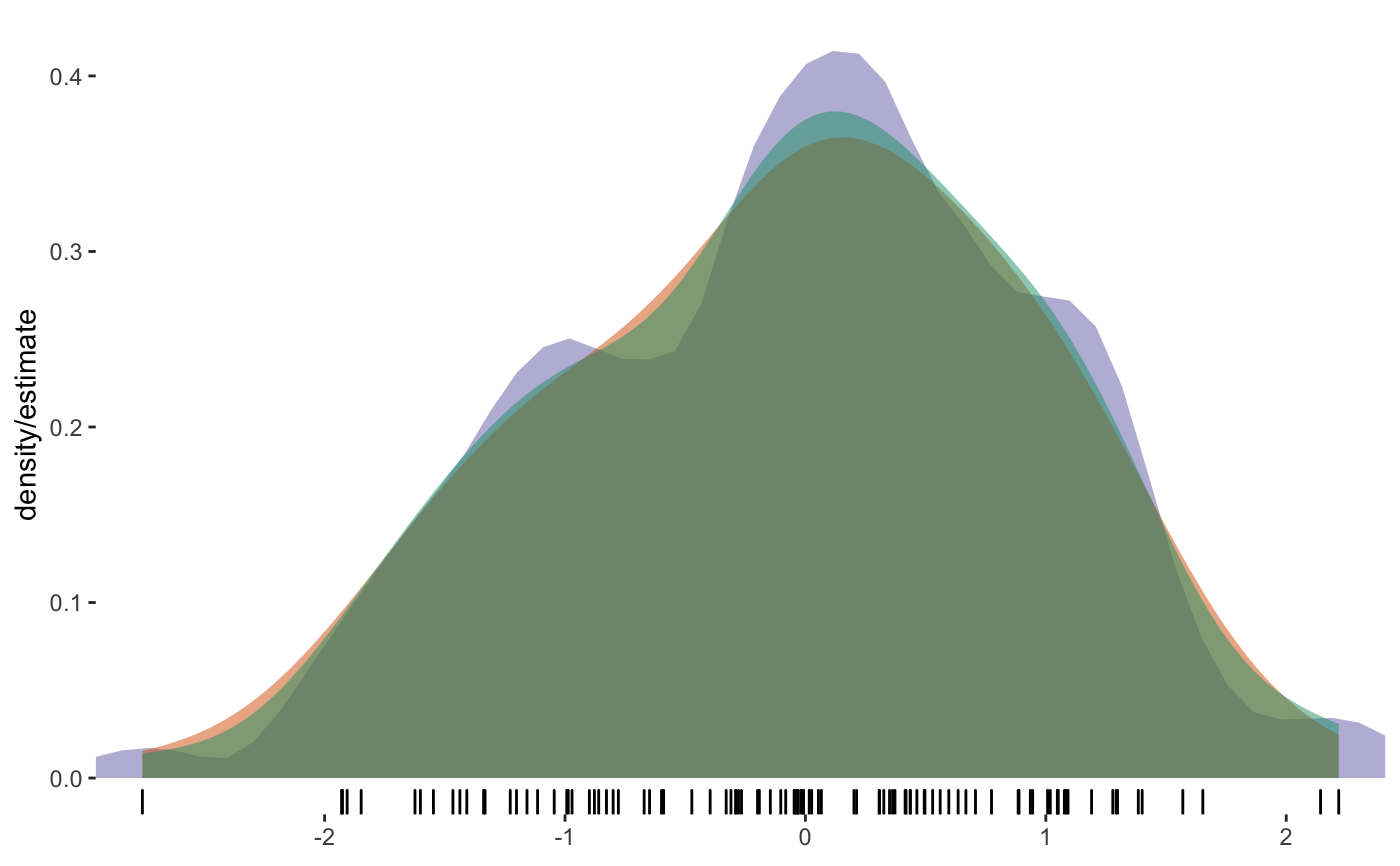
# compare
library(gridExtra)
set.seed(1492)
dat <- data.frame(x=rnorm(100))
grid.arrange(ggplot(dat, aes(x)) + stat_ash(),
             ggplot(dat, aes(x)) + stat_bkde(),
             ggplot(dat, aes(x)) + stat_density(),
             nrow=3)
#> Estimate nonzero outside interval ab.
#> Bandwidth not specified. Using '0.43', via KernSmooth::dpik.

cols <- RColorBrewer::brewer.pal(3, "Dark2")
ggplot(dat, aes(x)) +
  stat_ash(alpha=1/2, fill=cols[3]) +
  stat_bkde(alpha=1/2, fill=cols[2]) +
  stat_density(alpha=1/2, fill=cols[1]) +
  geom_rug() +
  labs(x=NULL, y="density/estimate") +
  scale_x_continuous(expand=c(0,0)) +
  theme_bw() +
  theme(panel.grid=element_blank()) +
  theme(panel.border=element_blank())
#> Estimate nonzero outside interval ab.
#> Bandwidth not specified. Using '0.43', via KernSmooth::dpik.